Haar wavelet
In mathematics, the Haar wavelet is a certain sequence of rescaled "square-shaped" functions which together form a wavelet family or basis. Wavelet analysis is similar to Fourier analysis in that it allows a target function over an interval to be represented in terms of an orthonormal function basis. The Haar sequence is now recognised as the first known wavelet basis and extensively used as a teaching example in the theory of wavelets.
The Haar sequence was proposed in 1909 by Alfréd Haar.[1] Haar used these functions to give an example of a countable orthonormal system for the space of square-integrable functions on the real line. The study of wavelets, and even the term "wavelet", did not come until much later. As a special case of the Daubechies wavelet, it is also known as D2.
The Haar wavelet is also the simplest possible wavelet. The technical disadvantage of the Haar wavelet is that it is not continuous, and therefore not differentiable. This property can, however, be an advantage for the analysis of signals with sudden transitions, such as monitoring of tool failure in machines.[2]
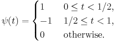
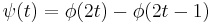
The Haar wavelet's mother wavelet function  can be described as
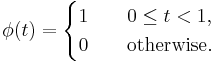
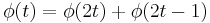
Its scaling function  can be described as
Contents |
Haar system
In functional analysis, the Haar systems denotes the set of Haar wavelets

In Hilbert space terms, this constitutes a complete orthogonal system for the functions on the unit interval. There is a related Rademacher system (named after Hans Rademacher) of sums of Haar functions, which is an orthogonal system but not complete.[3][4]
The Haar system (with the natural ordering) is further a Schauder basis for the space ![L^p[0,1]](/2012-wikipedia_en_all_nopic_01_2012/I/753faea37a4cd277395f93e7a7e3d728.png) for
for 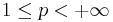 . This basis is unconditional for p > 1.
Haar wavelet properties
The Haar wavelet has several notable properties:
- Any continuous real function can be approximated by linear combinations of
 and their shifted functions. This extends to those function spaces where any function therein can be approximated by continuous functions.
 - Any continuous real function can be approximated by linear combinations of the constant function,
 and their shifted functions.
 - Orthogonality in the form
-
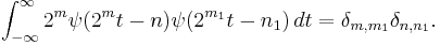
- Here δi,j represents the Kronecker delta. The dual function of is itself.
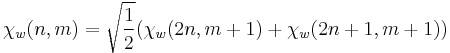
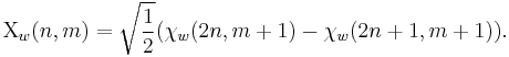
- 4. Wavelet/scaling functions with different scale m have a functional relationship:
- 5. Coefficients of scale m can be calculated by coefficients of scale m+1:
- If
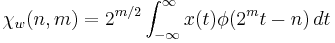
- and
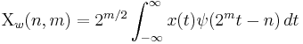
- then
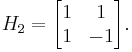
Haar matrix
The 2×2 Haar matrix that is associated with the Haar wavelet is
Using the discrete wavelet transform, one can transform any sequence 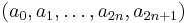 of even length into a sequence of two-component-vectors
 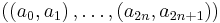 . If one right-multiplies each vector with the matrix
  , one gets the result
 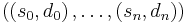 of one stage of the fast Haar-wavelet transform. Usually one separates the sequences s and d and continues with transforming the sequence s.
If one has a sequence of length a multiple of four, one can build blocks of 4 elements and transform them in a similar manner with the 4×4 Haar matrix
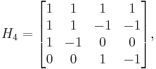
which combines two stages of the fast Haar-wavelet transform.
Compare with a Walsh matrix, which is a non-localized 1/–1 matrix.
Haar transform
The Haar transform is the simplest of the wavelet transforms. This transform cross-multiplies a function against the Haar wavelet with various shifts and stretches, like the Fourier transform cross-multiplies a function against a sine wave with two phases and many stretches.[5]
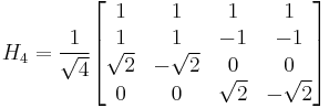
The Haar transform is derived from the Haar matrix. An example of a 4x4 Haar transformation matrix is shown below.
The Haar transform can be thought of as a sampling process in which rows of the transformation matrix act as samples of finer and finer resolution.
Compare with the Walsh transform, which is also 1/–1, but is non-localized.
See also
Notes
- ^ Haar, Alfred (1910). "Zur Theorie der orthogonalen Funktionensysteme". Mathematische Annalen 69 (3): 331–371. doi:10.1007/BF01456326.
- ^ Lee, B.; Tarng, Y. S. (1999). "Application of the discrete wavelet transform to the monitoring of tool failure in end milling using the spindle motor current". International Journal of Advanced Manufacturing Technology 15 (4): 238–243. doi:10.1007/s001700050062.
- ^ "Orthogonal system". Encyclopaedia of Mathematics. http://eom.springer.de/O/o070380.htm.
- ^ Shen, Gilbert G. (2001). Wavelets and Other Orthogonal Systems. Boca Raton: Chapman. ISBN 1584882271.
- ^ The Haar Transform
References
- Haar A. Zur Theorie der orthogonalen Funktionensysteme, Mathematische Annalen, 69, pp 331–371, 1910.
- Charles K. Chui, An Introduction to Wavelets, (1992), Academic Press, San Diego, ISBN 0585470901
External links
- Free Haar wavelet filtering implementation and interactive demo
- Free Haar wavelet denoising and lossy signal compression